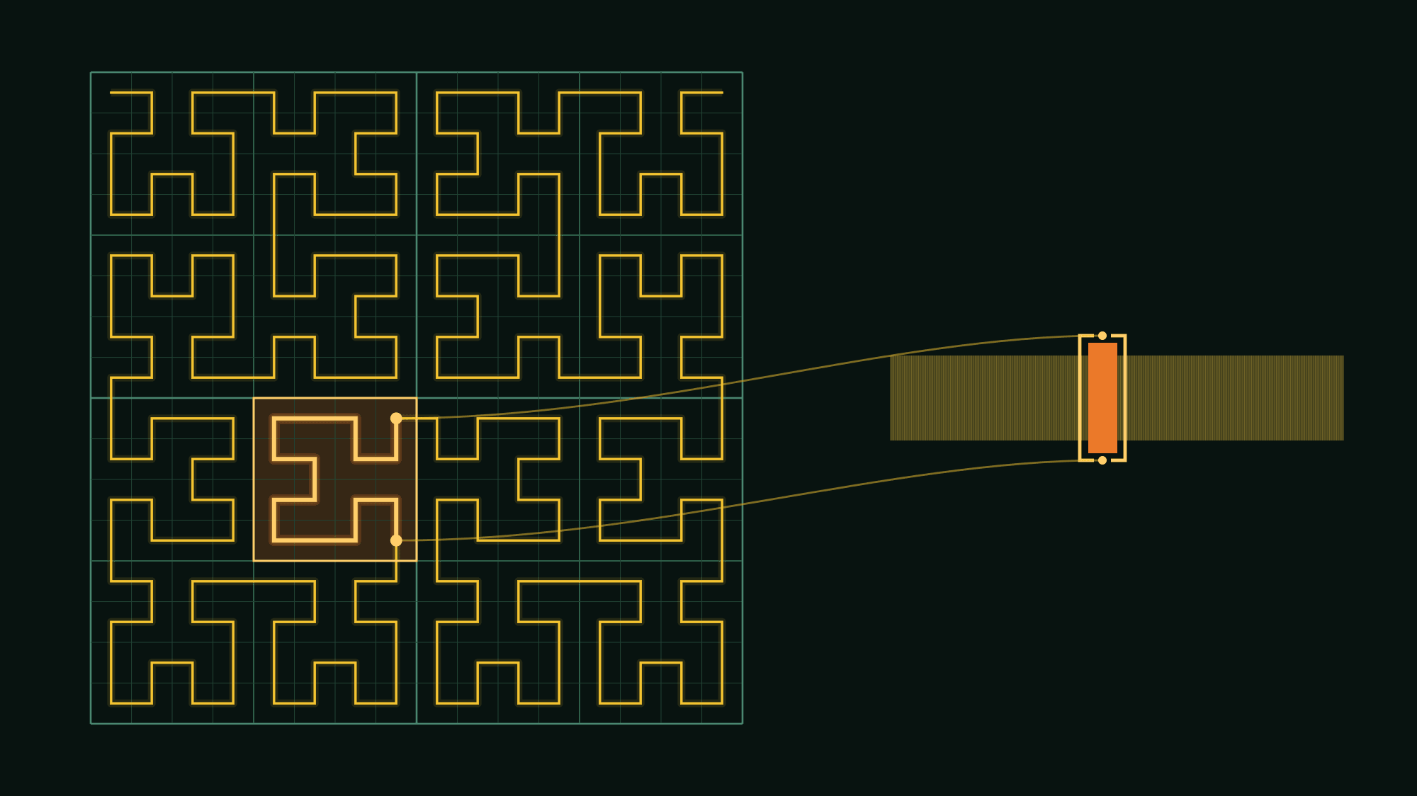
One S2 face as a quadtree, walked in Hilbert order. A contiguous block of cells (amber) is also a contiguous run of cell IDs, so a 2D region becomes a single integer interval [rangemin, rangemax].
• Coding • 25 min read
The nearest hospital to every place on Earth, in a single S2 range query
How to build an S2 index once, to then resolve distance and containment for every place on Earth in seconds
How far is the nearest hospital, for every place on Earth? At first, this sounds like a distance problem with billions of pairs to check. However, with the right tools, it isn’t a distance problem at all: with S2 indexing it’s the same query as which country, region, and locality contains this point? We can solve it with a plain integer range check against a single index.
Last week I was advising a client whose geo pipeline was getting slower every week. Their team had started with the obvious approach: given a few hundred thousand points and several hundred thousand polygons, for each point they scanned every polygon to find the one that contained it. As the input size grew, they watched the nightly batch pipeline become considerably slower and were running out of options.
As we sketched applicable approaches on a whiteboard, I realized I was drawing a picture I’d drawn before, a decade before at Google. The trick, using S2 geometry to turn spatial joins into key joins, is one of the most elegant and underrated primitives I’ve come across: the kind of indexing idea that, like Ukkonen’s suffix trees, collapses an apparently quadratic problem into something nearly linear.
The problem I was solving back then had the same shape but on a different application: the typical price of a hotel stay anywhere on Earth, any night of the year, served at 10ms latency, which required precomputing everything via batch pipelines. One step had to associate every hotel with every named place that might contain it: neighborhood, town, city, region, POI.
Written naively, that step is a cartesian product. Given H hotels and R regions, generate all H x R pairs and only keep the ones where the hotel falls inside the region’s polygon.
I’d built it as a Flume pipeline, computing summaries for every night of the year over data that already lived distributed across several storage backends. Running it on Flume was justified by the layout of the data, the multitude of prices we had, and the 365-day time dimension. However, joining points-against-polygons was always within reach of one machine. The primitive, the indexing trick at the heart of it, never needed a cluster around it.
To demonstrate it, I wanted to solve a fresh public-data version of that same problem on a pretty typical machine: an AMD Ryzen 9 7900 desktop (12 cores, 64 GB of RAM). The question I picked: where on Earth is your nearest hospital? Its naive form is 437 billion pairs. The S2 index collapses it to a single integer range-join: about an hour to build the index, and then the answer for every locality on Earth comes back in seconds. This post is the story of how.
The worst place to get injured
If you live on the Kerguelen archipelago (a French sub-Antarctic research outpost halfway between Madagascar and Antarctica) and you need a hospital, the nearest one is 3,362 km away, on Rodrigues Island in Mauritius. That’s farther than New York to Los Angeles. And it’s the loneliest result in a worldwide leaderboard of localities ranked by distance to their nearest healthcare facility, covering every place on Earth that anyone has put on the map.
The top of the leaderboard is unsurprising: the top three are all settlements on Kerguelen, the next seven are all Tuamotu atolls in French Polynesia. Interestingly, both are French overseas territories; together they sweep the entire global top 10 because:
- each small atoll is its own locality polygon,
- they really are extraordinarily remote, and
- France maps them well.
The last point was interesting: the underlying map data is a treasure, but has varying coverage by country. I suppose it’s due to a combination of factors, one of which being how active the local mapping community is. I guess it makes sense considering how much of it comes from OpenStreetMap volunteers.
A more interesting exploration asks the question per country, restricted to countries most readers will recognize. Click any row to see the actual location on OpenStreetMap.
| Country | Locality | km |
|---|---|---|
| Russia | Dikson, Arctic Ocean coast | 2,901 |
| Canada | Read Island, Northwest Territories | 2,264 |
| United States | Adak, Aleutian Islands, Alaska | 1,546 |
| Greenland (Denmark) | Nanortalik, southern Greenland | 1,171 |
| Australia | Mundrabilla, Nullarbor Plain | 631 |
| China | 黑瞎子岛镇, Bolshoy Ussuriysky Island | 584 |
| United Kingdom | Rockall, North Atlantic islet | 503 |
| Mauritania | Akdernit, Sahara | 365 |
| Madagascar | Beroboka Nord, western coast | 245 |
| Brazil | Oriximiná, Amazon interior | 230 |
| Mali | Tin Zaouatine, Algerian border / Sahara | 219 |
| Argentina | Sierra Colorada, Patagonia | 173 |
| Japan | Kitadaitōjima, remote Pacific island | 165 |
| Chile | Natales, Patagonia / Magallanes | 153 |
| Mexico | Progreso, Yucatán | 125 |
| Italy | Ustica, volcanic island | 57 |
| France | Île-de-Sein, Brittany | 45 |
A few things this list reveals (I had to look up every single one of them except for Ustica):
- The UK’s most-isolated mapped locality is Rockall: a tiny rocky islet in the North Atlantic, contested between four countries, with a Royal-Marines-occupied flagpole. So small, it turns out, that nobody lives on it at all (more on that below).
- China’s is Bolshoy Ussuriysky: a river island the PRC and Russia split between them in 2008.
- Australia’s Nullarbor Plain at 631 km is genuinely remote; the Outback is really isolated.
- Italy and France show what well-covered countries look like: the most-isolated locality is a tiny offshore island just ~50 km from the nearest hospital. That’s what most of Europe looks like.
Behind every entry on that table is one integer per locality, half a million of them, classified against every healthcare POI in Overture (the open global map dataset, introduced below), every (locality, POI) pair a potential great-circle distance. The primitive that makes this possible at scale is S2 cell indexing, originally built in the mid-2000s to power Google Maps. The same primitive simultaneously answers a different-looking question (what country, region, and city does each hospital belong to?) from the same index. That’s the part this post is built around.
The hotels-to-cities problem, again
The Flume pipeline from my memory was a hotels-to-cities job: for every (hotel, place) pair, answer is this hotel inside this place? The pipeline in my demo works for both hospitals-to-administrative-units and hospitals-to-radius-bands. S2 cell indexing makes these problems tractable by turning geographic questions (is point P inside polygon Q?) into an integer-key question (is the integer P′ in the sorted set Q′?). Then, a sort-merge pass handles the rest and the shape of the problem goes from quadratic-on-geometry to linear-on-integers.
I wanted to apply the lesson to a fresh problem with public data and real-world stakes, and settled for these two facets:
- Distance to the nearest hospital is something everybody understands. Mapping every hospital on Earth to every country, region, locality it belongs to, at the same time, is the same question as the hotels-to-cities use case from my experience.
- How far is the nearest hospital from each locality is the same question shape, just with distance bands instead of admin levels.
And S2’s hierarchy makes those two kinds of “level” indistinguishable to the algorithm. That’s the surprise from the beginning, spelled out: distance and containment are the same query: let’s see how.
S2 in one paragraph
S2 partitions the surface of the Earth into a quadtree of cells. Key principles:
- every cell has a unique 64-bit integer ID;
- every cell has a parent at the next coarser level;
- every leaf cell at level 30 (about 1 cm²) is the descendant of exactly one cell at every level above it;
- it’s possible to walk the S2 hierarchy all the way up to six face cells.
This strict parent-child invariant — that every leaf has a unique ancestor at every level — is what makes S2 special. It lets us encode every cell as an interval [range_min, range_max] over leaf-cell IDs. A leaf L is contained in cell C if and only if range_min(C) ≤ L ≤ range_max(C). One integer-interval check, no geometry, and it works at any level, on any cell, against any leaf. The whole post is built on this one trick.
Each S2 Cell ID is positional. Three bits pick one of six cube faces, then two bits per level pick one of four children, and a final 1 bit marks where the cell stops. A coarser cell is therefore a binary prefix of all its descendants:
cell C 011 10 00 11 · 1 · 0000…0
range_min(C) 011 10 00 11 · 0000…00 · 1
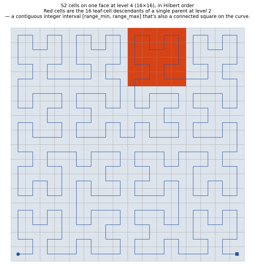
range_max(C) 011 10 00 11 · 1111…11 · 1Every leaf under C shares the prefix 011 10 00 11 and varies only in the bits below it, from all-zeros to all-ones. That span is the interval [range_min, range_max], and “is this leaf inside this cell?” becomes “does this integer fall in that range?”. It’s prefix matching, the same trick a router uses on a CIDR block. The Hilbert ordering shown below adds a separate property on top: nearby cells get nearby IDs, so a whole region covers into just a few of these intervals instead of thousands.
The data
The dataset I used for the demo is Overture Maps, a public release of Meta’s, Microsoft’s, AWS’s, and TomTom’s joint cleanup and merge of OpenStreetMap, Microsoft Building Footprints, and assorted proprietary data. As of the May 2026 release it has 54 million POIs and 1.07 million administrative polygons, all openly available as Parquet on S3, byte-range-readable with no auth required.
I pulled the global tile to my workstation via the overturemaps CLI in a few minutes. From that, the input set for this post:
- 770,440 healthcare POIs:
hospital,medical_center,emergency_room,urgent_care_clinic. This deliberately excludes pharmacies, dental clinics, and specialist offices. You could reproduce the same approach with any other type of POI. - 567,307 localities: cities, towns, villages, wards.
- ~4,700 regions, ~380 country polygons (some countries have multiple polygons in the source, such as overseas territories, exclaves, and disputed islands, which get rolled up to one ISO code at aggregation time).
Those three admin levels add up to ~572,000 polygons: a subset of Overture’s 1.07 million administrative polygons.
Mapping every POI to every admin level, in one pass
For each admin polygon (country, region, locality) we then build its cell-union: the smallest set of S2 cells whose union covers the polygon. Each cell carries an INTERIOR / BOUNDARY tag. INTERIOR cells are entirely inside the polygon; BOUNDARY cells straddle its edge. The construction is a single call to S2’s RegionCoverer, wrapped to also tag each cell:
from geo.s2_covering import cover_polygon

# `polygon` is a shapely geometry for one admin region.
# `cover_polygon` returns a mixed-level cell-union: small cells along
# the boundary, big cells inside the bulk.
tagged = cover_polygon(polygon, min_level=4, max_level=12, max_cells=200)

rows = [
    (admin_id, c.range_min, c.range_max, c.tag == "INTERIOR")
    for c in tagged
]
Building the cell-union table for those ~572,000 admin polygons produces ~5.7 million rows in 36 minutes on the workstation. Each row is a small struct: (admin_id, range_min, range_max, is_interior).
For each healthcare POI, I compute its leaf cell, a 64-bit integer. All 770k of them take four seconds.
Then a single SQL range-join in DuckDB (conceptually similar to SQLite, but for analytical work on columnar data):
SELECT poi.id, admin.id, admin.subtype
FROM poi_leaves poi
JOIN unified_cell_union admin
  ON poi.leaf BETWEEN admin.range_min AND admin.range_max
That’s the whole spatial join.
What’s impressive is that it works across all admin levels at once. It returns ~5.6 million candidate (POI, admin) pairs in under a second:
- ~965k INTERIOR matches are auto-confirmed: leaf is inside an INTERIOR cell, no further work needed.
- ~4.7M BOUNDARY matches need a real polygon-contains check; ~3.3M survive.
The refinement is the only place geometry comes back into the loop. To keep it cheap, group the candidates by admin polygon: load each polygon’s geometry once, then call shapely.contains against every POI that landed in one of its boundary cells:
from shapely.geometry import Point

confirmed = []
for admin_id, group in boundary_candidates.groupby('admin_id'):
    poly = admin_polygons[admin_id]      # loaded once per admin
    confirmed.extend(
        (poi_id, admin_id)
        for poi_id, lon, lat in group.itertuples(index=False)
        if poly.contains(Point(lon, lat))
    )
Polygon loads dominate the runtime; the contains calls are cheap because the admin polygon was already simplified upstream of the index. ~4.7M candidates → ~3.3M confirmed in a few minutes.
Total: ~4.2 million confirmed (POI, admin) pairs, across country and region and locality, in 6 minutes of compute.
To make the join concrete, take a real hospital: Bergamo’s Ospedale Papa Giovanni XXIII, at roughly (45.6917° N, 9.6692° E). Its S2 leaf cell ID is 5,152,488,575,548,925,233. Each admin polygon is a union of many cells; the one whose interval contains that integer is its matching cell. A cell and its interval are the same object: a cell at level k is exactly the leaf range [range_min, range_max]. The three matching cells:
| Admin polygon | Matching cell | range_min | range_max |
|---|---|---|---|
| Italia (country) | level 6 | 5,152,117,973,711,847,425 | 5,152,680,923,665,268,735 |
| Lombardia (region) | level 7 | 5,152,399,448,688,558,081 | 5,152,540,186,176,913,407 |
| Bergamo (locality) | level 11 | 5,152,488,509,130,407,937 | 5,152,489,058,886,221,823 |
Three nested intervals on the same number line, and the hospital’s leaf cell ID falls inside all three. The SQL above resolves country, region, and locality containment with one BETWEEN per row, against one unified table. The usual way to answer “which polygon contains this point?” is a spatial index like an R-tree, the structure behind PostGIS and most geo databases. But an R-tree covers one layer of polygons at a time, so all three admin levels mean three separate indexes and three separate tree searches. Three integer comparisons against one table replace all of it.
The cell-union skews heavily toward BOUNDARY cells. Real admin polygons have long, jagged perimeters relative to their area, and RegionCoverer adaptively subdivides only the edge cells: each level of refinement turns ~1 straddling parent into ~2 straddling children, so a few edge cells at coarse levels balloon into many leaf BOUNDARY cells at max_level. Meanwhile the polygon’s bulk gets covered by a handful of large INTERIOR cells.
That skew doesn’t slow the join down, though. The range-join itself is just BETWEEN comparisons, so it doesn’t care how the cells are tagged. The only real cost is the BOUNDARY refinement, and most of those checks land on leaf cells at max_level, where the geometries are small and shapely.contains runs in microseconds. INTERIOR cells help at the margin, auto-confirming the POIs that fall in a polygon’s bulk, but the join is fast mainly because even the boundary path is cheap: a tiny leaf, an already-simplified polygon, a microsecond contains call.
The refinement work scales with polygon perimeter at max_level, not with area.
Distance is just another kind of hierarchy
Now the harder-looking question: how far is the nearest hospital from each locality? The naive solution is to treat it as a nearest-neighbor problem: for each locality, scan all hospitals, find the closest. Even with a spatial index it’s a different kind of problem from the admin-rollup join.
Is it though?
For each healthcare POI, we can build a spherical cap at each radius band (within 1 km, within 5 km, within 15 km, within 30 km, within 100 km) and cover each cap with S2 cells. The construction in S2 is about as short as it gets:
import s2sphere
EARTH_RADIUS_KM = 6371.0

center = s2sphere.LatLng.from_degrees(poi.lat, poi.lon).to_point()
cap = s2sphere.Cap.from_axis_angle(
    center,
    s2sphere.Angle.from_radians(radius_km / EARTH_RADIUS_KM),
)
cells = region_coverer.get_covering(cap)
Here:
get_coveringis the same primitive used for the admin polygons;Capis just a shapeRegionCovererknows how to cover.
Cap.from_axis_angle. On a flat plane the same region would be a disk; wrapping the plane onto the sphere turns it into the cap, which keeps the bands honest out to the 100 km radius.Then we take the per-radius union across all 770k POIs. The result is five cell-unions (one per radius band), each tagging the part of the planet that’s within that radius of some hospital.
Then, for each locality, we take its representative point’s leaf cell and ask: what’s the smallest band whose cell-union contains me? That’s its isolation distance.
The check is identical to the admin one: leaf BETWEEN range_min AND range_max. The hierarchy now spans distance scales instead of administrative scales, and the algorithm doesn’t know or care about the difference. I see that as more proof of the elegance in the S2 design: country / region / locality / 1 km / 5 km / 30 km are all the same kind of thing to the index. They are all representable as nested cell-unions over a quadtree, and queryable with a single integer-interval check.
This is where S2 separates from H3, Uber’s hexagonal grid system, and from R-trees. R-trees can do range queries but need one tree per question: four levels of hierarchy = four trees, four traversals. H3 can index polygons but its parent-child relation is approximate, so a multi-level union breaks the integer-interval trick. S2’s strict quadtree parent-child invariant is the property that makes the same primitive work for both kinds of hierarchy.
Here are the cell counts per band, after normalization:
| Radius | Cells (after normalize) |
|---|---|
| 1 km | 1,575,449 |
| 5 km | 724,157 |
| 15 km | 317,056 |
| 30 km | 129,497 |
| 100 km | 11,021 |
Bigger radii merge into coarser parents, yielding fewer cells for the same fidelity. Building all five bands across 770k POIs took 30 minutes; classifying 567k localities into bands took 30 seconds.
A booby-trap
The first version of the global leaderboard had Archipel des Crozet at 2,008 km. Being unfamiliar with many of these locations, I decided to do some spot-checking. Crozet is a sub-Antarctic French island group in the southern Indian Ocean, about as far from anything as land gets, so I expected a big number. But 2,008 felt too low: Crozet to Cape Town is 2,400 km, Crozet to Madagascar is 2,400 km, and there’s nothing in between. A hospital can’t sit closer than the nearest land, I thought. So where was this 2,008-km hospital?
A query of my data gave me the answer: at coordinates (-30.75°, 63.63°), the middle of the open Indian Ocean. Querying that location in Overture’s data turned up:
서울병원 (Seoul Hospital), country=KR
A Korean hospital tagged ~10,000 km from Korea, due to a geocoding error somewhere upstream in the OSM ingest. That phantom POI was the “nearest hospital” pulling Crozet down to 2,008 km. It did worse damage next door: it also sat ~2,150 km from Kerguelen, well inside Kerguelen’s true ~3,360 km, so it had also quietly bumped the genuine top results off the board. Three more ghosts turned up at similar mid-ocean coordinates, each understating how isolated some real place is.
The fix is one filter, against the same table we built for the join:
-- Keep POIs whose leaf falls inside some country polygon.
-- Misgeocoded ocean POIs never match because no country range covers
-- the open ocean.
SELECT DISTINCT poi.id
FROM poi_leaves poi
JOIN unified_cell_union admin
  ON poi.leaf BETWEEN admin.range_min AND admin.range_max
 AND admin.subtype = 'country';
That’s the same BETWEEN primitive, restricted to one admin level. The index doesn’t need to know what a “country” is; it just trusts the cell-union for subtype = 'country'. After the filter, Kerguelen reclaims the top three and Crozet settles at its real ~2,400 km (nearest hospital in Madagascar): still extraordinarily remote, just below the Kerguelen and Tuamotu tier at the top of this post.
The lesson, more useful than the leaderboard: even with a clean algorithm and public data on a workstation, the first answer is wrong in interesting ways. The question shape is right; the data has booby-traps; you find them by looking at outliers and asking “does this make sense geographically?”
You’ll often hear advice that in any data problem (whether it’s for ML or data analysis), spending time eyeballing the data for patterns and outliers pays off. This is one more example of that.
See it
The interactive map above zooms through three layers of the same join focused on my home country: Italy. 20 regioni, 8,577 comuni, and 12,579 healthcare POIs. Polygon fills are colored by what fraction of contained comuni are within 5 km of healthcare: blue good, red bad, cream in the middle. Hover any feature for its per-area stats. Toggle “Density” to switch from access to healthcare-POIs-per-km².
Why Italy specifically? Of course I have ties to the country, but beyond that, there are more interesting reasons.
While the algorithm is universal, the input data isn’t: Overture’s locality coverage is dense across Italy (every comune mapped) and several other countries, but patchy elsewhere. Showing the join over Italy keeps the demo interesting and realistic: every visible polygon is a real comune with a real population, not a hole in OSM’s coverage. When I worked on this problem at Google, we were also dependent on the quality of data from Google Maps, and we knew that some countries were better mapped than others.
A few patterns the Italian view makes obvious:
- The alpine arc (Valle d’Aosta, Trentino, the northern fringe of Lombardia and Veneto) reads warmer: small mountain comuni without their own hospital, leaning on the valley town next door. An interesting follow-up study might be considering driving distance, which I’d expect to affect POI accessibility even more.
- Po Valley, Tuscany, Campania around Naples, the Adriatic coast read cool: dense comune mosaic, dense hospital coverage.
- Sardinia and Sicily show internal isolation: interior mountain comuni warm, coastal comuni cool.
- Zoom in far enough and the POI dots light up: deep red for hospitals, blue for emergency rooms.
See the join structure itself
Flip on Show S2 cells in the toolbar. The choropleth gets overlaid with the actual S2 cell-union used by the join: green cells are INTERIOR (entirely inside the polygon, auto-confirmed in the range query), orange cells are BOUNDARY (straddle the edge, refined via shapely.contains). At low zoom you see the per-regione cell-union; at z7–z8 it hands off to the per-comune cell-unions, the same parent-child hand-off the algorithm relies on. Around that zoom level you can briefly see both layers on top of each other: a Lombardia-tier cell sitting above the Milan / Monza / Lodi comune cells it contains. That visual nesting is the integer-interval check from the SQL block earlier in the post.
One thing the overlay makes visible: the INTERIOR/BOUNDARY split looks completely different depending on what you count. Barely 1% of the cells in Italy’s cell-union are INTERIOR; nearly all the rest trace the jagged comune and regione edges. That sounds like the algorithm’s “fast path” is doing almost no work, but the matches skew far more INTERIOR than the cells do, because POIs cluster in the bulk of polygons, not on their edges, exactly as the join section above described.
What the answer doesn’t (and can’t) say
Four caveats deserve more than a footnote:
OSM coverage varies by country. The dataset’s tagging fidelity isn’t uniform. Italy’s espresso bars are tagged bar and not coffee_shop; Vietnam tags every cà phê; Thailand tags every clinic; rural Russia barely tags anything. For isolation distance, this means the answer is an upper bound wherever coverage is thin: when we say “120 km to the nearest hospital,” the truth is “120 km to the nearest hospital that someone bothered to map.” That’s the right answer to what does the public dataset say. It’s not the answer to where are the actual hospital deserts without continued investment in mapping ground truth as open data.
Density is partly a tagging-density story. The “densest healthcare” leaderboard is dominated by Bangkok wards (top entry: 254 healthcare POIs per km², four of the top five are in central Bangkok), then Delhi, Jakarta, Taipei, Seoul, Saigon. Bangkok’s medical-tourism culture and high small-clinic density are real. But Thai OSM mappers are also unusually thorough. The dataset’s leaderboards are always partly a leaderboard of map quality.
Outright vandalism happens. OSM is open; some entries are jokes. Greenland’s top-isolated locality in the raw data came back as a Skibidi-meme joke name that someone added to the map. Same problem as the misgeocoded ocean POIs: once you look at the answers, you find them. (Filter that one and the next entry, a real Inuit settlement on the east coast, slides up.) The shape of the problem is the same: a public dataset’s leaderboard is downstream of the public dataset’s quality, and you treat it as data not as truth.
A locality isn’t necessarily inhabited. When I looked into the UK’s lonely winner, Rockall, it turned out to have no permanent population at all. Nothing is wrong with the data, though: Overture has an optional population field, but it’s sparse, and the locality subtype only asserts that someone put a named place on the map, not that anyone lives there.
Locality coverage is wildly uneven across countries, which is why the live demo in this post is Italy. Overture inherits OSM’s country-level mapping density: Italy has 8,577 mapped comuni, France 36,752 communes, Germany 22,967. Greece has 178. Within the US, Massachusetts is fully tiled with mapped places; Virginia is full of gaps. A global choropleth at city zoom reads great over Western Europe and becomes visibly patchy elsewhere, not because the algorithm breaks, but because the input data is uneven. The interactive in this post uses Italy because every visible polygon is a real comune with a real population.
Why this is an S2 post and not just a “use a spatial index” post
The cell-set inner join, on its own, doesn’t distinguish S2 from any other spatial index. R-trees do range queries. H3 cells can index polygons. DuckDB’s plain ST_Contains is already quite fast at this scale on its own: for a single-level point-in-polygon problem, a generic spatial join would land in the same ballpark.
What S2 buys with its versatility, and what this post is built to show, is one index, every scale at once:
- The same cell-union table resolves country and region and locality for any point: single integer-interval lookup against a unified table.
- The same primitive resolves what 1 km / 5 km / 30 km radius am I in for any point: same lookup, separately-built but structurally identical table.
- The two kinds of “level” are the same kind of thing to the algorithm. R-trees would need four trees and four traversals. H3 has parents; that’s not the issue. The issue is that H3 cell IDs across resolutions live in disjoint integer spaces. The encoding embeds the resolution in the ID itself, so a leaf cell at res 9 and its res-5 ancestor are unrelated integers. There’s no equivalent to S2’s
[range_min, range_max]that lets a single leaf ID be range-checked against a cell at any coarser level. With H3 you can do lookups, but only at one fixed resolution at a time. S2’s strict quadtree invariant, that every cell at every level is representable as an integer interval over leaf IDs, is what makes the multi-resolution unified table work.
Concretely, here’s what that costs visually. The same patch of Lombardia, covered two ways:
![Lombardia covered two ways. On the left, S2's mixed-level cell-union: 59 cells at levels 5–9. Three large green INTERIOR cells tile the polygon's bulk; the remaining 56 BOUNDARY cells (orange, finer) handle the edges. Mixing levels is legal because S2's quadtree guarantees each cell's [range_min, range_max] over leaf IDs cleanly contains all its descendants, so coarse and fine cells live in the same integer-indexed table. On the right, H3 at two resolutions overlaid: res 4 (15 large blue hexes) and res 5 (97 red strokes laid on top). The red boundaries cross the blue ones; the smaller hexes do not nest inside the bigger ones. A res-4 cell well inside Lombardia has a 14.3% symmetric-difference with the union of its 7 res-5 children: children spill out and leave gaps. That's why H3 can't do the S2 trick of mixing resolutions in one cell-union table.](/_astro/s2_vs_h3_lombardia.Db7VYosd.png)
S2’s mixed-level union is a clean tiling: a handful of large interior cells, a band of small boundary cells, no gaps and no overlaps. H3’s geometry can’t deliver that: pick one resolution and you get a sensible cover; try to mix two and the cell boundaries don’t agree. The hex grid is the wrong shape for a strict quadtree invariant.
Cell counts across the three nested admin polygons make the same argument numerically:
| S2 (mixed levels) | H3 res 5 (~8.5 km) | H3 res 7 (~1.2 km) | H3 res 9 (~174 m) | |
|---|---|---|---|---|
| Italia (country) | 178 | 1,701 | 83,322 | 4,081,854 |
| Lombardia (region) | 59 | 97 | 4,653 | 227,466 |
| Bergamo (locality) | 16 | 1 | 8 | 380 |
The S2 union uses cells at levels 4–8 for Italy, 5–9 for Lombardia, 8–12 for Bergamo: bulk gets covered by a few large cells, only the edges need fine ones, all coexisting in the same table because the integer intervals at the leaf level let them. H3 has to commit to one resolution: at res 5 Bergamo is a single hexagon (unresolvable), at res 7 Italy needs 83,000 hexagons in the index, at res 9 the index is unworkable. H3’s compact() helps some (it can fold contiguous fine cells back into parents) but the resulting set still isn’t a range-comparison primitive, and the lookup remains set-membership at a chosen resolution. You can build a working spatial join with H3; you can’t build this particular multi-scale unified-index join with it. That’s the structural property S2 gives you, and the post is built around it.
Concretely: the unified cell-union table over 572k admin polygons is 46 MB. The five radius-band cell-unions over 770k POIs total ~70 MB. Both indexes are tiny, and building them is the only slow part: the admin cell-unions take 36 minutes, the radius bands 30, so the indexes are ready in about an hour. Everything after that is a query. The range-join that resolves country, region, and locality for all 770k POIs returns in under a second; classifying every one of the 567k localities on Earth into a nearest-hospital band takes 30 seconds. The one query-side step that costs minutes, the boundary refinement, is geometry-loading, not the join.
Which loops back to the opening. I used a distributed batch job via Flume for the original problem at Google, not because the algorithm needed one but because the data was huge. Here the entire pipeline (both indexes, the joins, the refinement, the aggregation) runs on a single CPU, no GPU, no cluster. A point-in-polygon question becomes an integer-interval question, and the rest is sort-merge. Build the index once, and the planet-scale query is seconds of work. The index is what did the real work, at fleet scale and on a desktop alike.
Reproduce
The code is at github.com/abahgat/s2-spatial-join (public, MIT-licensed). All data sources are open and auth-free. End-to-end on a workstation, from raw Overture tiles to the finished leaderboard, runs in under two hours. Almost all of that is the one-time index build (the admin cell-unions and the radius-band cap coverings, the latter dominated by the finest-level band), not the queries, which answer in seconds once the index exists.
uv sync
uv run overturemaps download -t place         -f geoparquet -o data/cache/world_places.parquet
uv run overturemaps download -t division_area -f geoparquet -o data/cache/world_divisions.parquet
uv run python scripts/bake_healthcare_world.py            # phases A–D: indexes
uv run python scripts/bake_healthcare_world_geojson.py # phase E: aggregate + leaderboardIf you want to ask the same kind of question of a different POI category (most isolated locality from a school, a pharmacy, a fire station, a bookstore, a coffee shop) the pipeline generalizes by changing one filter line, and runs in the same amount of time. The S2 index doesn’t care what kind of POI you put in it. That, more than any specific number, is the point.
The engineering leader I was coaching: their pipeline is now an integer-interval check too. They didn’t need a cluster either.